2 Details of the Paper
2.1 Model
- There are \(M\) LTCI markets that are defined by a geographical state and calendar year
- In each market, there exists a unit mass of potential consumers and many potential insurers
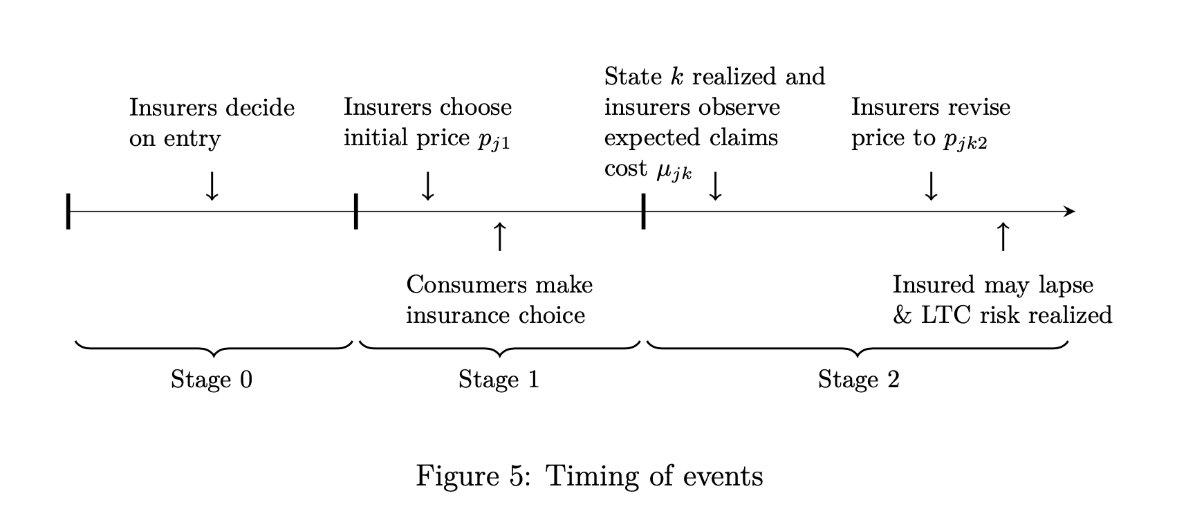
- There are three stages in the model (see Figure 5)
- In stage 0, insurers decide whether to enter the market based on the entry cost and the expected profit
- In stage 1, insurers set an initial price for their LTCI contract
- In stage 2, the uncertainty about aggregate risk is resolved, and insurers revise their price determined in the first stage. Consumers with private LTCI might lapse their contract, and LTC utilization takes place in the end.
2.1.1 Fringe firms’ entry decision
- Fringe firms will enter the market if their expected profit is equal to or greater than their entry cost \(c^{e}\), which follows the CDF denoted by \(G\). - Once fringe firms enter, they will respectively earn the profit of
\[ \max \{\frac{1}{n_{J}} \Pi^{∗}_{J} −c^{e}, 0 \} \]
2.1.2 Firms’ initial pricing and consumers’ insurance choice
- At the beginning of stage 1, the market consists of \(J − 1\) major firms and one representative fringe which is the collection of fringe entrants.
- Let \(j \in \{1, 2,..., J \}\) index insurers where j$ = J$ means the representative fringe.
- Insurer \(j\)’s profit in stage 1 is
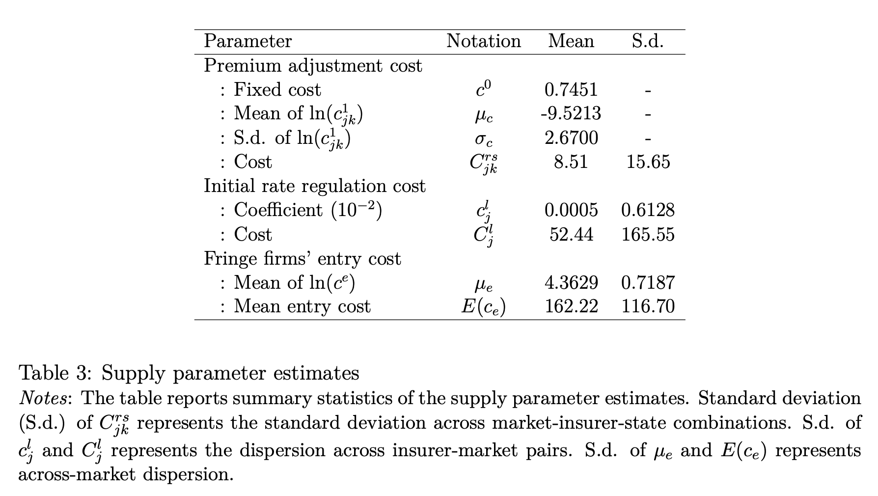
\[ \Pi_{j1} = p_{j1}s_{j1} − C_{j}^{l}(p_{j1} − \tilde{\mu_{j}}) \]
- Consumer \(i\)’s flow utility from contracting with insurer \(j\) in stage 1 is
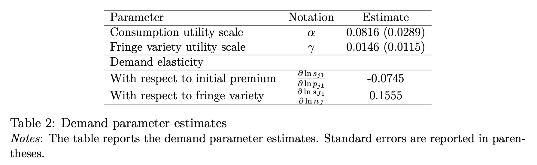
\[ \tilde{u}_{ij1} = \alpha u(y_{i}− p_{j1}) + \gamma I(j = J) \ln(n_{J}) + \xi_{j} + \varepsilon_{ij} \]
- If consumer \(i\) does not purchase any private LTCI, then her utility in stage 1 is given by \[ \tilde{u_{i01}} = \alpha u(y_{i}) + \varepsilon_{i0} \]
2.1.3 Firms’ revised pricing
There are \(K\) possible aggregate states of the world in stage 2, and each state happens with probability \(\Pi_{k}\) where \(k = 1, ..., K\)
When state \(k\) is realized, insurers learn that the expected claims cost from their existing cohort of consumers is equal to \(\mu_{jk}\).
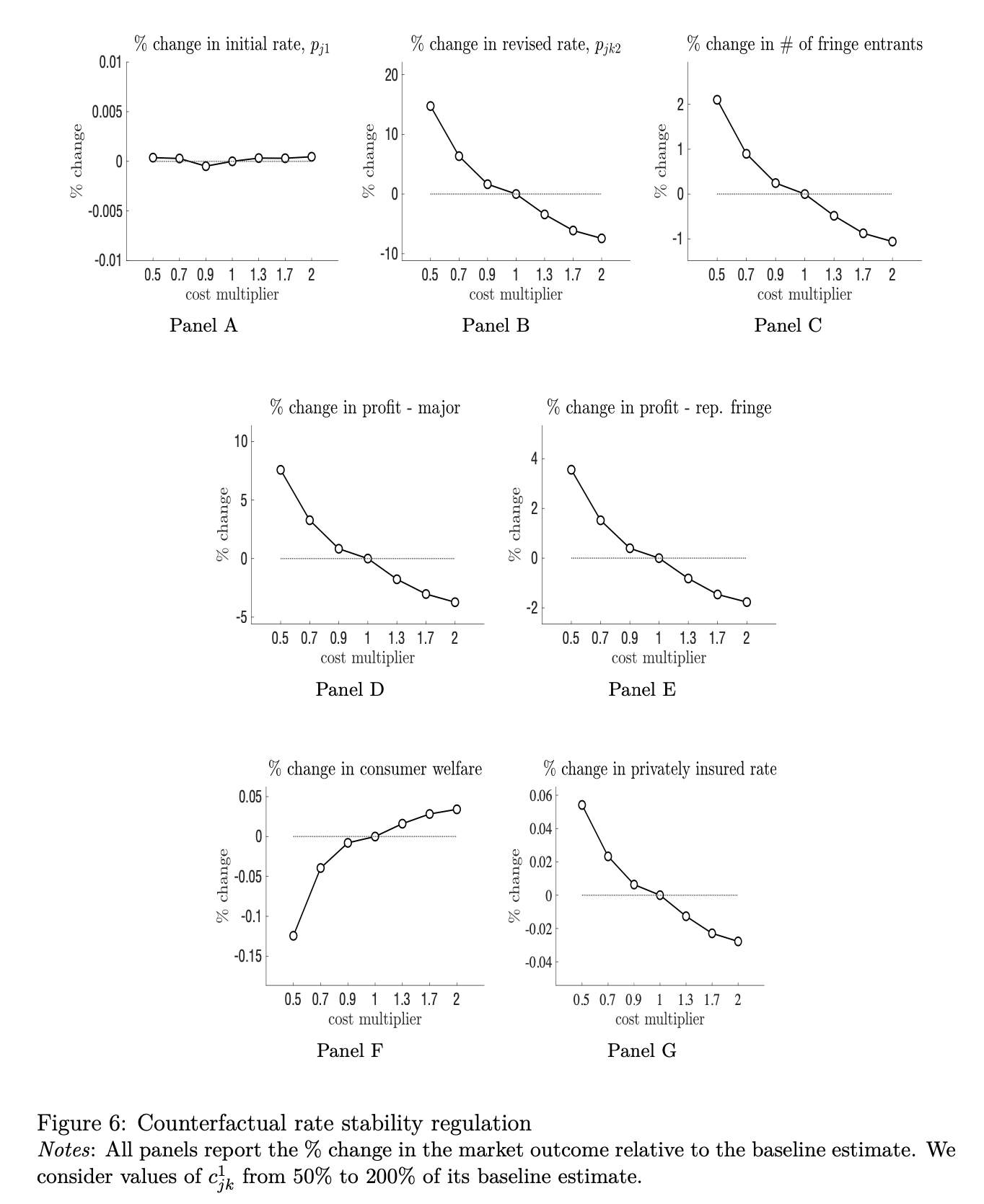
Insurers then decide whether to increase the initial premium, and if so, by how much. Insurers are subject to the rate adjustment cost \(C^{rs}_{jk}(p_{j1} ,p_{jk2})\), which represents the cost associated with revising the premium from \(p_{j1}\) to \(p_{jk2}\) when the realized state is \(k\) in stage 2.
Insurer \(j\)’s profit from the second stage when the realized state is \(k\) is \[ \Pi =(p_{jk2} − \mu_{jk})s_{jk2} − C^{rs}_{jk}(p_{j1} ,p_{jk2}) \]
When the realized state is \(k\), consumer \(i\)’s expected utility from holding the contract sold by insurer \(j\) is
\[ \tilde{u}_{ijk} = (1 − \delta_{k})u_{ijk, stay} + \delta_{k}u_{ik, lapse} \]
- The utility from retaining the current contract is given by
\[ u_{ijk, stay} = \alpha u(y_{i}−p_{jk2}) + \gamma I(j = J)\ln(n_{J}) + \xi_{j} \]
- The utility from terminating the contract is given by \[ u_{ik,lapse} = \int_{\lambda} \alpha u(y_{i} − oop(\lambda, y_{i}))f_{k}(\lambda) d\lambda \]
2.1.4 Equilibrium
Consumers in the first period make insurance purchase decisions to maximize their lifetime utility.
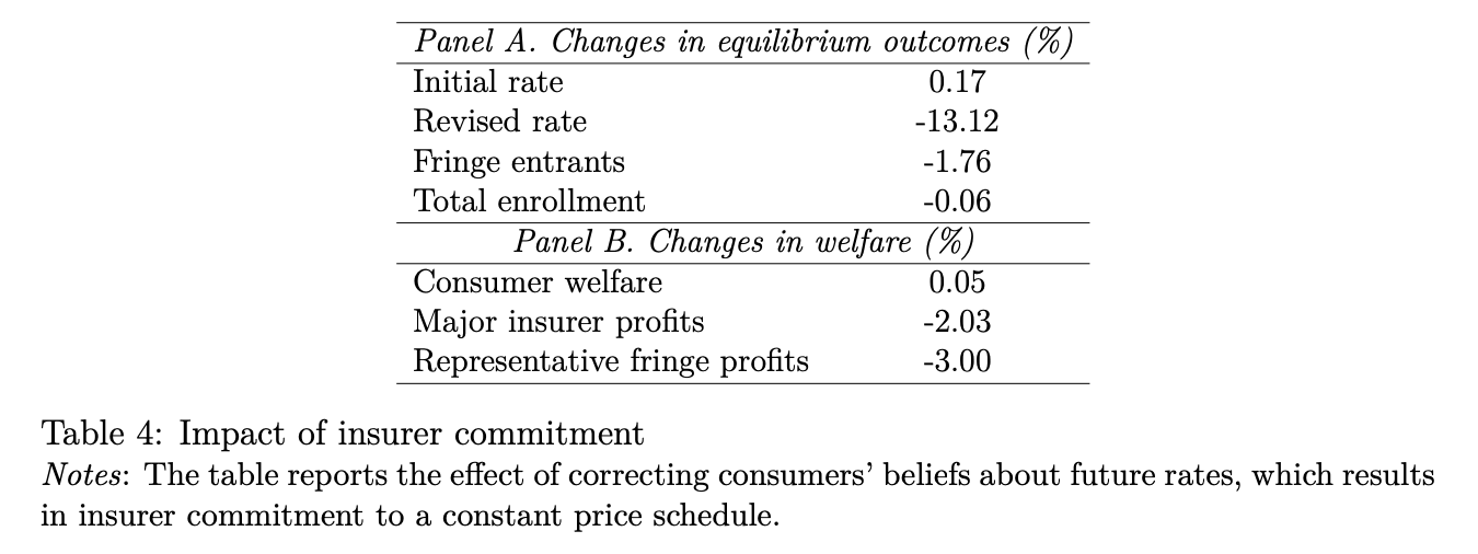
Consumer \(i\)’s expected lifetime utility from contracting with insurer \(j \in \{1, ..., J \}\) is \[ \tilde{v}_{ij} = \alpha u(y_{i} − p_{j1}) + \gamma I(j = J) \ln(n_{J}) + \xi_{j} + \beta_{c}\sum_{k} \pi_{k}((1 − \delta_{k})u_{ijk, stay} + \delta_{k}u_{ik, lapse}) + \varepsilon_{ij} \]
The consumer’s expected lifetime utility from not purchasing any insurance is \[ \tilde{v}_{0} = \alpha u(y_{i}) + \beta_{c} \sum_{k} \pi_{k} u_{ik, lapse} + \varepsilon_{i0} \]
If \(j^{∗}\) is the chosen option by consumer \(i\), then \(j^{∗} = \mathop{\rm argmax}\limits_{j = 0, 1, ..., J} \tilde{v}_{ij}\).
Insurers’ problem can be solved backwards. In stage 2, given the realized state \(k\), each insurer \(j\) chooses the revised premium by maximizing its state-specific profit: \[ \Pi^{∗}_{jk2} = \max_{p_{jk2}}(p_{jk2} − \mu_jk)s_{jk2} − C^{rs}_{jk}(p_{j1} ,p_{jk2}) \]
Given the optimal sequence of \(\{ p_{jk2} \}^{K}_{k = 1}\) which is a function of the initial premium \(p_{j1}\), insurer \(j\) in stage 1 chooses \(p_{j1}\) to maximize its profit over the lifetime of LTCI contracts: \[ \Pi^{∗}_{j} = \max_{p_{j1}} p_{j1}s_{j1} −C^{l}_{j}(p_{j1} - \tilde{\mu}_{j}) + \beta_{f}\sum_{k}\pi_{k}\Pi^{∗}_{jk2} \]
In stage 0, a fringe firm with entry cost \(c^{e}\) will enter the market if \[ c^{e} \leq \frac{1}{n_{J}} \Pi^{∗}_{J} \]
We characterize a Nash equilibrium in each market that consists of the vector of premiums \((p_{j1},\{ p_{jk2} \}^{K}_{k = 1})\) for each insurer \(j\) and the number of fringe insurers \(n_{J}\) that solve above equations.